The bayesrules package has a set of functions that support exploring Bayesian models from three conjugate families: Beta-Binomial, Gamma-Poisson, and Normal-Normal. The functions either help with plotting (prior, likelihood, and/or posterior) or summarizing the descriptives (mean, mode, variance, and sd) of the prior and/or posterior.
The Beta-Binomial Model
We use the Beta-Binomial model to show the different set of functions and the arguments.
Prior
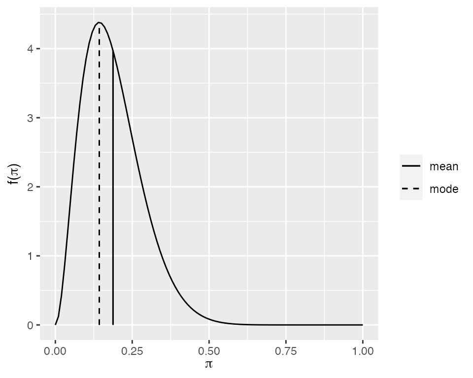
plot_beta(alpha = 3, beta = 13, mean = TRUE, mode = TRUE)
#> Warning in geom_segment(aes(x = mean, y = 0, xend = mean, yend = dbeta(mean, : All aesthetics have length 1, but the data has 2 rows.
#> ℹ Please consider using `annotate()` or provide this layer with data containing
#>   a single row.
#> Warning in geom_segment(aes(x = mode, y = 0, xend = mode, yend = stats::dbeta(mode, : All aesthetics have length 1, but the data has 2 rows.
#> ℹ Please consider using `annotate()` or provide this layer with data containing
#>   a single row.
summarize_beta(alpha = 3, beta = 13)
#>     mean      mode         var         sd
#> 1 0.1875 0.1428571 0.008961397 0.09466466
Likelihood
In addition, plot_binomial_likelihood() helps users
visualize the Binomial likelihood function and shows the maximum
likelihood estimate.
plot_binomial_likelihood(y = 3, n = 15, mle = TRUE)
#> Warning in geom_segment(aes(x = max, xend = max, y = 0, yend = dbinom(success, : All aesthetics have length 1, but the data has 2 rows.
#> ℹ Please consider using `annotate()` or provide this layer with data containing
#>   a single row.
Prior-Likelihood-Posterior
The two other functions plot_beta_binomial() and
summarize_beta_binomial() require both the prior parameters
and the data for the likelihood.
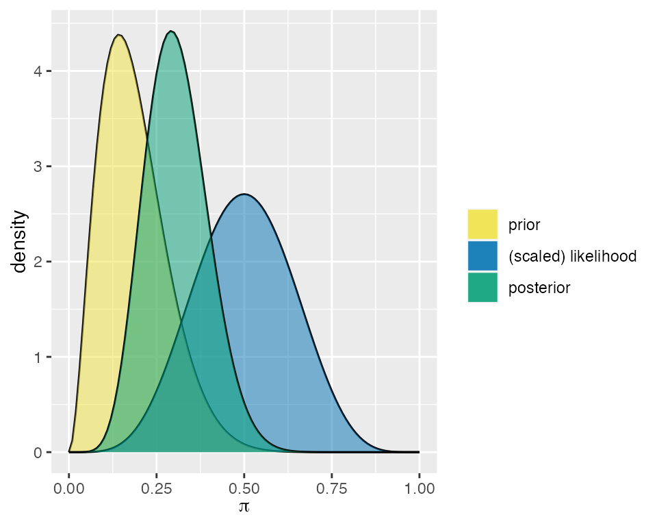
plot_beta_binomial(alpha = 3, beta = 13, y = 5, n = 10,
                   prior = TRUE, #the default
                   likelihood = TRUE,  #the default
                   posterior = TRUE #the default
                   )
summarize_beta_binomial(alpha = 3, beta = 13, y = 5, n = 10)
#>       model alpha beta      mean      mode         var         sd
#> 1     prior     3   13 0.1875000 0.1428571 0.008961397 0.09466466
#> 2 posterior     8   18 0.3076923 0.2916667 0.007889546 0.08882312
Other Conjugate-Families
For Gamma-Poisson and Normal-Normal models, the set of functions are
similar but the arguments are different for each model. Arguments of the
Gamma-Poisson functions include the shape and
rate of the Gamma prior and sum_y and
n arguments related to observed data which represent the
sum of observed data values and number of observations respectively.
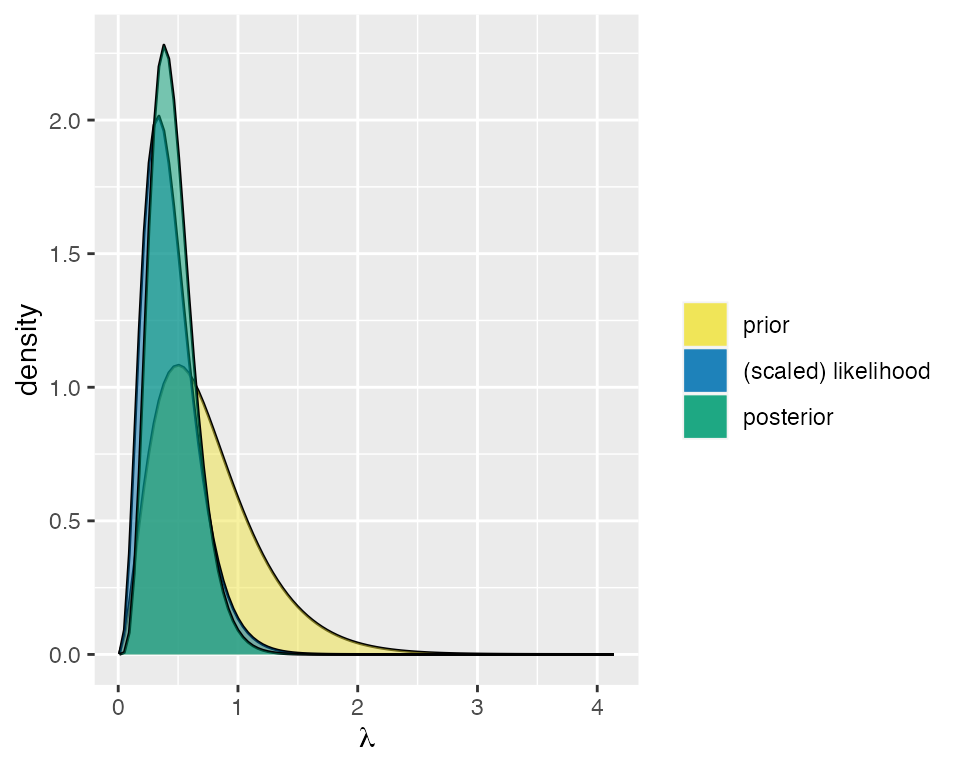
plot_gamma_poisson(
  shape = 3,
  rate = 4,
  sum_y = 3,
  n = 9,
  prior = TRUE,
  likelihood = TRUE,
  posterior = TRUE
)
For the Normal-Normal model functions, the prior Normal model has the
mean and sd argument. The observed data has
sigma, y_bar, and n which
indicate the standard deviation, mean, and sample size of the data
respectively.
summarize_normal_normal(mean = 3.8, sd = 1.12, sigma = 5.8, y_bar = 3.35, n = 8)
#>       model     mean     mode      var        sd
#> 1     prior 3.800000 3.800000 1.254400 1.1200000
#> 2 posterior 3.696604 3.696604 0.966178 0.9829435